This is the script I knocked up tonight. There are many improvements to be made but as a quick hack I am pleased to say it works and produced the graph above. I also want to use the Cairo package to get the graphic output antialiased and prettied up.
Update: Well it looks like my blog trashes the formatting on my script so I will put an image of it up tomorrow instead to replace the mess below.
#################################################################
#################################################################
## ##
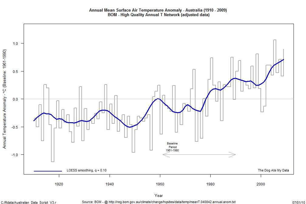
## Step chart of NASA GISS annual temperature anomaly (C) data ##
## ##
#################################################################
#################################################################
###############################
# Step 1: SETUP SOURCE FILE #
###############################
rm(list=ls())
link <- "C:\\Rdata\\Bom_Yrly_Anom_1910_2009.csv"
script<- " C:/Rdata/Australian_Data_Script_V3.r"
#############################################################
# Step 2: READ DATA FROM CSV FILE WITH FIRST ROW HEADINGS #
#############################################################
my_Data <- read.table(link,
sep = ",", dec=".", skip=0,
row.names = NULL, header = T,
colClasses = rep("numeric", 2),
na.strings = c("", "*", "-", -99.99, 99.9, 999.9))
#############################
# STEP 3: MANIPULATE DATA #
#############################
# Construct chart title - nothing to manipulate this time
Title <- paste("Annual Mean Surface Air Temperature Anomaly - Australia (1910 - 2009) \nBOM - High Quality Annual T Network (adjusted data)" )
#########################
# STEP 4: CREATE PLOT #
#########################
## GRAPHIC PARAMETERS
win.graph(width = 10.5, height = 7, pointsize = 12) ### Sets size of graphics window ###
par(bg = "white"); # sets background colour, default = transparent
par(las = 1) # Sets Y axis label orientation to vertical, set text font sizes
par(cex.main=0.8); par(cex.sub=0.7); par(cex.lab = 0.8); par(cex.axis =.75);
## HIGH LEVEL GRAPHIC FUNCTION CALL
#usr <- par("usr") ,
#rect(usr[1], usr[3], usr[2], usr[4], col="cornsilk", border="black"),
plot(Anomaly ~ Year, my_Data,
ylim = c(-1.25,1.25),
type=c("s"),
col = "dark grey",
lwd = 2, #line width
xlab = "Year",
asp = "FULL",
bty ="o",
ylab = expression(paste("Annual Temperature Anomaly - ",degree, "C (Baseline: 1961-1990)")),
main = Title,
sub = "Source: BOM - @ http://reg.bom.gov.au/climate/change/hqsites/data/temp/meanT.040842.annual.anom.txt")
## LOW LEVEL GRAPHIC FUNCTION CALL
lines(lowess(my_Data$Anomaly ~ my_Data$Year, f=0.1),col = "blue", lwd = 3)
arrows(1961,-1.0, 1990, -1.0, code = 3, angle = 20, col = "dark grey")
abline(h=0, col = "grey") # o.o horizontal line
text(1965, -.990, "Baseline\n Period\n1961-1990", cex = 0.6, pos=3)
text(1931, -1.20, "LOESS smoothing, q = 0.10", cex =0.65, pos =1)
points(c(1910,1921), c(-1.3,-1.3), col="blue", type = "l", lwd = 2)
text(2005, -1.2, "The Dog Ate My Data", cex=0.65, pos=1)
## Add script name & print date to chart
my_date <- format(Sys.time(),"%d/%m/%y ")
mtext(script, side=1, line = -1, outer = T, adj = 0, cex = 0.65)
mtext(my_date, side = 1, line = -1, outer = T, adj = 1, cex = 0.7)
###################
# STEP 5: CLOSE #
###################
# todo


5 comments:
Put a PRE & /PRE tag around the whole region, and it will format as monospace with preserved linebreaks
Thanks Sierra. I will repost the code with the proper tags tonight. Much appreciated.
You also need to replace the angle brackets within the code with < or > entities, or they will be misinterpreted as HTML. Usually better in these cases to link to a separate file containing the raw text, in which case you don't need to encode characters for presentation within an HTML page.
Yep I see what you mean. The code seems to be displayed now however due to the line lengths I used and the format of the blog page it is still difficult to read. I'll have to set up files to link to as I have some better scripts just about ready to go when I get a chance to finalise them. More to follow shortly on the blog.
To prevent long lines of code from wrapping within the relatively narrow column, try adding this to your PRE tag:
<pre style="overflow:scroll">
Post a Comment